Engineering laboratory / Spring 2026
Experimental Instrumentation & Validation
Sensor calibration, data acquisition, and model validation across five mechanical engineering experiments.
The BU ME 310 laboratory sequence covered electrical measurement, strain, temperature, aerodynamic drag, and mechanical vibration. Each study used calibration and uncertainty analysis to convert sensor output into a physical result, then compared that result with expected behavior or an analytical model.
- Course
- BU ME 310
- Period
- Spring 2026
- Format
- Four laboratory studies and a final team project
- Areas
- Sensor calibration, signal conditioning, data acquisition, uncertainty, and model validation
- Tools
- LabVIEW, MATLAB, NI DAQ, oscilloscope, DMM, and wind tunnel
Instrumentation workflow
Each experiment followed the same path from physical behavior to a reported result: transduction, signal conditioning, data acquisition, calibration, uncertainty analysis, and model comparison.
- 01
Physical behavior
Temperature, strain, force, pressure, or displacement
- 02
Transduction
A sensor converts the behavior into an electrical signal
- 03
Conditioning
A divider, bridge, amplifier, or resistor makes the signal usable
- 04
Acquisition
An instrument or DAQ records repeated voltage measurements
- 05
Validation
Calibration, uncertainty, and a physical model turn voltage into evidence
Signal measurement and strain validation
The first study covered oscilloscope triggering, peak and RMS quantities, the signal generator's 50-ohm output, RC phase and step response, and power-supply grounding. These methods were used to configure and verify the instruments in later studies.
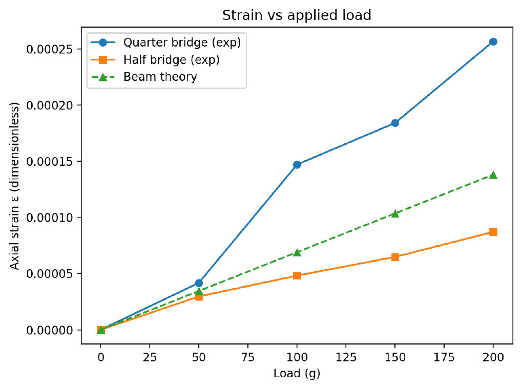
The strain study extended that foundation into a complete calibrated system. A Wheatstone bridge converted resistance change into differential voltage, an amplifier increased the signal for acquisition, and beam theory provided an independent reference. The amplifier gain measured 101.62 V/V, and the bridge balanced at 9,885 ohms against a 9,886-ohm prediction.
Half-bridge troubleshooting
A half bridge should have produced roughly twice the sensitivity of the quarter bridge. It instead produced a smaller signal and a large baseline offset. The result was traced to the measurement setup rather than the cantilever response, with bridge-arm assignment, a weak gage connection, and a damaged lead identified as likely causes.
Calibrating two temperature sensors
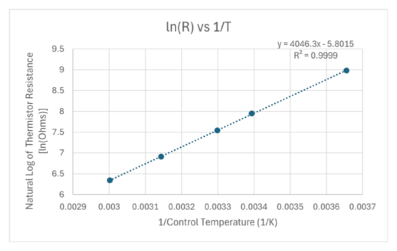
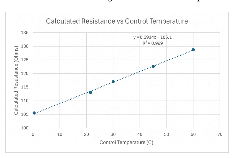
Controlled-temperature baths were used to calibrate a thermistor and an RTD as complete measurement systems. A DMM provided direct resistance checks, the DAQ captured repeated voltage samples, and the oscilloscope revealed time-varying noise that an average alone could hide.
The thermistor was more sensitive and strongly nonlinear. Its transformed response was almost perfectly linear, producing a thermistor constant of approximately 4,046 K. The RTD response was steadier and nearly linear, making it the better basis for estimating the unknown bath at 40.5 ± 2.45 °C.
Aerodynamic drag measurement
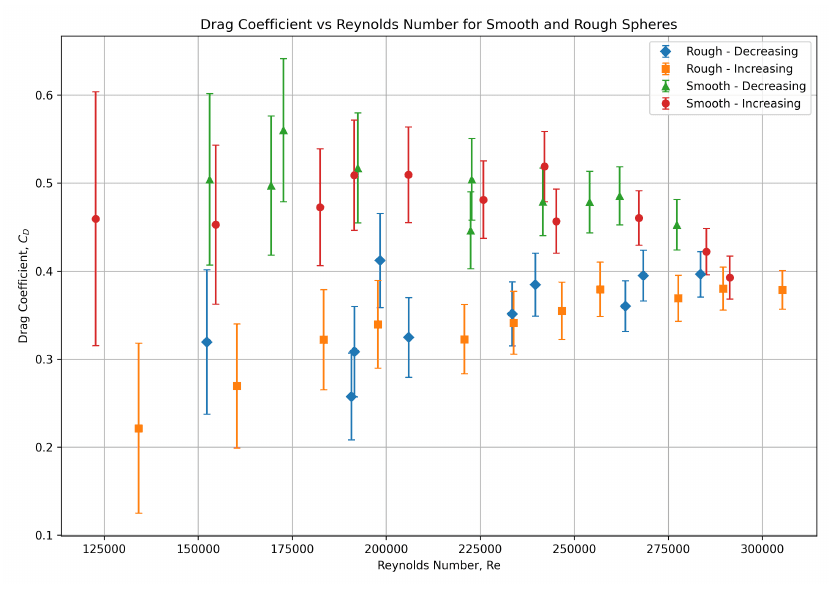
Load-cell voltage was calibrated to force, pressure-transducer voltage to dynamic pressure, and dynamic pressure to airspeed. Those relationships produced Reynolds number and drag coefficient for smooth and rough spheres while uncertainty was propagated through the result.
The smooth sphere remained near the expected pre-drag-crisis range, roughly 0.45 to 0.52. The rough sphere generally produced lower coefficients, about 0.22 to 0.40, consistent with an earlier boundary-layer transition and delayed separation. The tunnel approached but did not sharply capture the smooth sphere's full drag crisis, so the conclusion stayed tied to the range the apparatus actually reached.
Final project
Identifying a weakly nonlinear oscillator
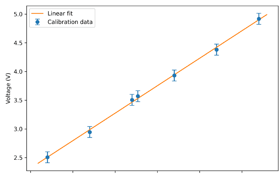
The final project combined the course's measurement methods into a single system. An optical proximity sensor measured the upper mass of a motor-driven spring-mass oscillator. A 500.668-ohm resistor converted the sensor's current output into voltage, a DMM supported setup and calibration, and an NI DAQ recorded the motion for analysis.
Optical measurement chain
Optical proximity sensor
Distance becomes a 4–20 mA current signal.
Current-to-voltage circuit
A measured resistor creates a DAQ-compatible voltage.
NI data acquisition
The top-mass response is sampled at 1,000 Hz.
Post-processing
Calibration, FFT estimates, peak timing, and curve fits recover motion and system constants.
Model comparison
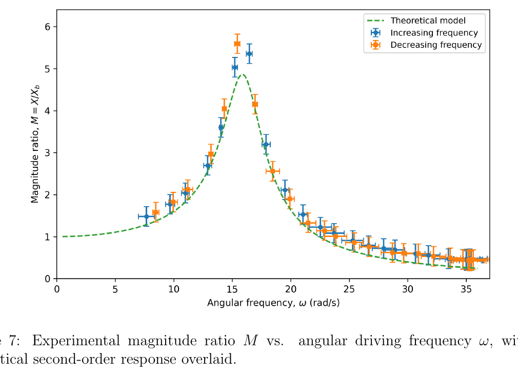
Motor settings were not assumed to map linearly to driving frequency. Each recorded signal was converted to displacement, centered, checked with an FFT, and refined from time-domain peak spacing. The measured response then rose sharply near resonance and fell at higher frequency, matching the expected second-order shape.
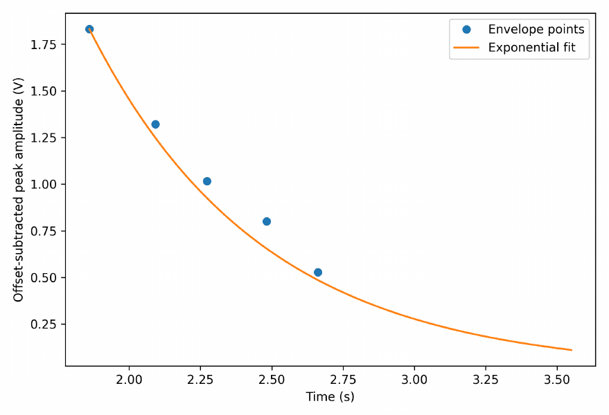
The increasing and decreasing sweeps did not overlap perfectly. Spring behavior, changing collar friction, non-sinusoidal Scotch-yoke motion, and motor loading all introduced behavior outside the ideal linear model. The free-decay estimate was therefore used for the final natural frequency and damping ratio because it relied on the direct decay of the system rather than judgment about the resonance peak.
- Upper moving mass
- 0.303 ± 0.0005 kg
- Spring constant
- 132.7 ± 5.4 N/m
- Natural frequency
- 16.04 ± 0.065 rad/s
- Damping ratio
- 0.1034 ± 0.0304
- Damping coefficient
- 1.31 ± 0.387 kg/s
Experimental studies
Signal measurement
Oscilloscope, multimeter, signal generator, and RC circuit
Established triggering, RMS, phase, step-response, and grounding methods used in later experiments.
Strain and deflection
Wheatstone bridges, bonded strain gages, and a differential amplifier
Compared cantilever strain and deflection with beam theory and traced an abnormal half-bridge response to the measurement setup.
Temperature calibration
Thermistor and RTD voltage-divider circuits
Separated nonlinear and linear sensor behavior, quantified uncertainty, and measured an unknown bath temperature.
Aerodynamic drag
Load cell, pressure transducer, pitot-static measurement, and wind tunnel
Mapped drag coefficient against Reynolds number and tested the effect of surface roughness on transition.
Dynamic system identification
Optical proximity sensor, current-to-voltage conditioning, and NI DAQ
Measured a weakly nonlinear oscillator, identified its dynamic constants, and compared its frequency response with a second-order model.
Outcome and reflection
The work progressed from learning individual instruments to designing and validating a complete transduction system. By the final project, raw voltage histories could be carried through a documented chain into displacement, frequency response, natural frequency, damping ratio, and uncertainty.
Differences between measurement and theory were evaluated as part of the result. Depending on the experiment, they indicated an instrument fault, a limit in the available operating range, or behavior excluded from the analytical model.